Having two different data sets, for example a customerslist and a productslist, and want to combine them to get a new list with all possible combinations of customers and products ?
The solution is pretty simple, feasible with MSExcelin a few minutes, and, even with thousands of entries, doesn’t require much effort – much less than copy pasting the second list for each value of the first list – this last solution would take hours with hundreds of entries.
In short :
Create a numeric identifier from 1 to the number of entries for each source file,
In the result file,
Create a numeric identifier (ID) in column A going from 1 to the multiplication of the count of first file entries and second file entries, creating as many lines as the combination of both data sets,
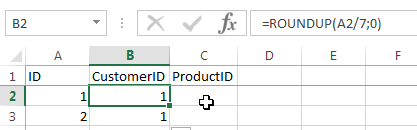
Add a column, enter this formula and expand it to the last line =ROUNDUP(A2/[Second file entries count];0)
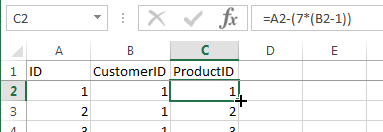
Add a column, enter this formula and expand it to the last line =A2-([Second file entries count]*(B2-1))
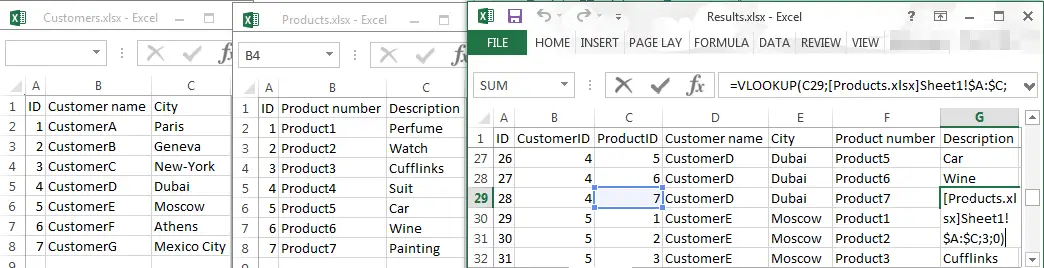
Add as many columns as you want to get from first and second files, and do vlookups on corresponding identifier in result file and source files
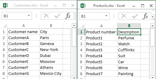
See below a full example, with a Customers list and a Products list
Two data sets to combine into one by creating all possible combinations
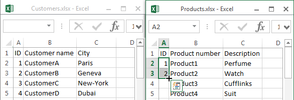
Start by creating identifiers in both file, by adding a column on the left, entering values 1 and 2 in the first two lines, selecting the two cells, moving the mouse cursor to the bottom-right corner on the selection, and double clicking on the + sign to expand the identifier increment to the last line.
Creation of first two identifiers and appearance of the expand function
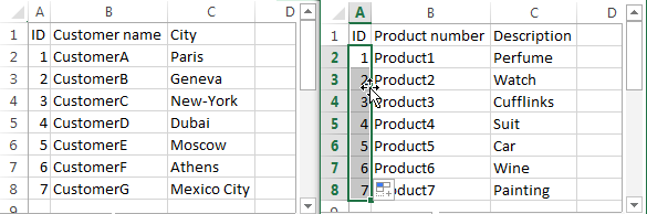
As a result, the identifiers have been incremented up to the last line.
Identifiers automatically incremented until the last line
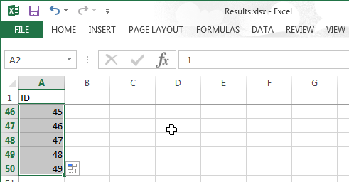
Take the maximum identifier numbers of both Customers (C) and Products (P). Create a new file, with a column identifier, and repeat the identifier expand operation, down to the line (C * P) + 1. In below example, 7 different values for Customers, and 7 for Products, resulting in 7 * 7 = 49 combinations, + 1 line to make up for the header line.
Result file with identifiers for all possibilities
In column B, we’ll put the P lines per Customer, as each of them will have one line per Product. This is done by using below formula in the sheet’s second line, and expanding it to the bottom (remember the double click on the + icon in the bottom-corner of the cell selection to do so)
=A2-([Second file entries count]*(B2-1))
Function roundup to repeat each first file identifier for as many second files entries
In column C, we’ll put a count for each of the Customers, from 1 to Products count. Same operation as before, with another formula (current line identifier minus the count reached for previous Customer line)
=A2-([Second file entries count]*(B2-1))
Restart the second file identifier count from 1 for each block of first file identifiers
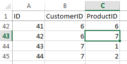
Check if it have worked. Customers are repeated P times, and for each of them, the Products identifier are repeated from 1 to P
Check that resulting file proposes all possible combinations
And that’s it ! Then, for each column you’d like to take over from Customers or Products file, add a new column, and perform a Vlookup on the corresponding identifier and source file.