Wondering how to make a table look good in MS Excel 2013?
Here are a few steps to help you, with a full example below :
Format as table, using Excelpredefined styles,
Copy formatting, from one cell to another,
Merge and center, when cell descriptions applies to several columns / lines,
Add borders, to visually distinguish easily important blocks,
Set text to bold, to visually notify important cells,
Format cells values, to properly display numbers, percentages, …
Resize columns to fit content.
You can always go further, but these easy and fast steps will quickly make your Exceltable look better.
Starting from a non formatted table, as seen below, you can see there’s a lot to improve.
Raw unformatted table
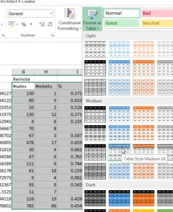
First step, apply some Exceltable to distinct subtables. Select them, and use the Format as Table option from Stylesbox in the HOME menu.
Format subtables as table
You might use Medium formats for content, and Dark format for a heading subtable, as shown in example.
Use another table format for heading subtable
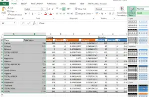
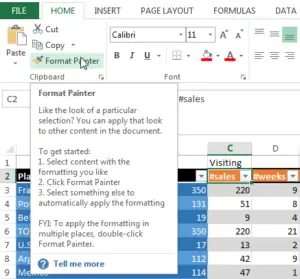
If you have extra cells, and want to apply the same style, select the cell from which the style should be copied, click on Format Painter from Clipboardbox in the HOME menu, and then click on the cells on which you want to copy the format.
Format painter to copy cell format
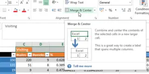
If several cells represent the same information, instead of copy pasting them, make sure the first cell of the selection (from the left for horizontal selection, or the top for vertical selection), select the contingent cells that should contain the same information, and apply the Merge & Centeroption from the Alignmentbox in the HOME menu.
Merge and center cells
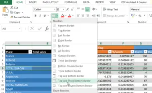
To make some blocks of information more obvious, for example subtotals and totals, select the corresponding line or column, and apply a Borderfrom the Fontbox in the HOME menu.
Apply borders to cell selection
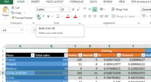
It might also be useful to format then in Boldfrom the same Fontbox in the HOME menu.
Format cells with bold text
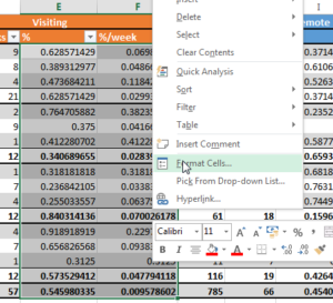
Some text might need to be reformatted, for example numbers only showing 2 decimals, or some numbers formatted as Percentage. Select the data you want to format, right click on the selection, and select the Format Cells… option.
Format cells as number / percentage …
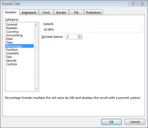
In that option, select the category you want to apply, and change the options to fit your needs, in our case Percentagewith 2 decimals.
Select cells format type (number, percentage, …)
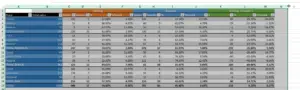
Then, select the columns, and when having the icon as shown on picture by pointing at the intersection of two columns identifier, double click to resize them all automatically.
Resize columns to fit content
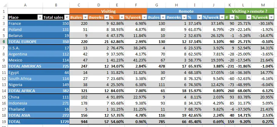
And voilà ! Your table should now look much better and you can now share it.